Controls

generate $\tau$ to get $\ddot{q}$

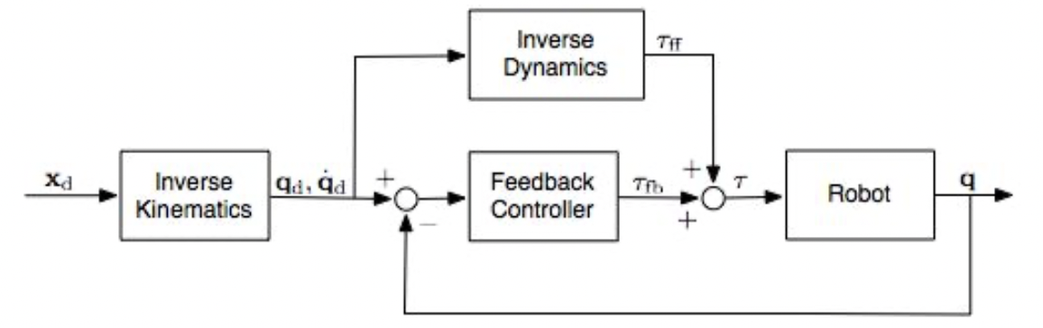
Feedforward control ( open loop )

Inverse Dynamics $\tau = M(q_d)\ddot{q}_d + C(q_d,\dot{q}_d)+G(q_d)$ Forward/Direct Dynamics $\ddot{q} = M(q)^{-1}(-C(q, \dot{q})-G(q)+\tau)$ eg. the pendulum system: $I\ddot\theta + k\dot\theta+rmg\theta = \tau$

Feedback steady-state error

Inverse dynamics control

Compare output $\ddot{q}$ with desired trajectory and correct. Let $\tau = \underbrace{k_p(\theta_d-\theta)}_{\text{spring}}\underbrace{-k_v\dot{\theta}}_\text{damper}$ to manipulate the dynamics of the system.

$I\ddot\theta + k\dot\theta+rmg\theta = \tau = -k_p(\theta_d-\theta)-k_v\dot{\theta}$ $\red{I\ddot\theta + (k+k_v)\dot\theta}+(rmg+k_p)\theta = k_p\theta_d$

System will end at $t \rightarrow \infty, (\ddot\theta=0,\dot\theta=0)$: $\theta=\frac{k_p}{\red{rmg} +k_p}\theta_d$

Because of gravity $rmg$ system will not reach target but will get close for large $k_p$. The steady state error is defined as: $e_{ss} = \theta_d(\infty)-\theta(\infty) = \frac{rmg}{rmg+k_p}$ steady state error is finite if $g\neq0$.

PID controller: (I sums up remaining error. Generally NOT safe for robots) $\tau = \underbrace{k_p(\theta_d-\theta)}_{\text{P:Proportional }}\underbrace{-k_v\dot{\theta}}_\text{ D:Derivative}+\underbrace{\red{k_i\int(\theta_d-\theta)dt}}_\text{I:Integral}$

More general: $\tau = K_P(q_d-q)-K_D(\dot q_d-\dot q)$ $e_{ss} = q_d-q=K_P^{-1}G(q)$ $K_P,K_D$ are diagnal matrices with each joint of value $k_{Pi},k_{Di}$.

Gravity compensation

PD control with gravity compensation(Safer than PID): $\tau = \underbrace{k_p(\theta_d-\theta)}_{\text{P:Proportional }}\underbrace{-k_v\dot{\theta}}_\text{ D:Derivative}+\underbrace{rmg\theta}_\text{gravity compensation}$

$I\ddot\theta + k\dot\theta+rmg\theta = \tau = -k_p(\theta_d-\theta)-k_v\dot{\theta}+rmg\theta$ $\red{I\ddot\theta + (k+k_v)\dot\theta} + k_p\theta = k_p\theta_d$

System will end at $t \rightarrow \infty, (\ddot\theta=0,\dot\theta=0)$: $k_p\theta=k_p\theta_d$ $e_{ss} = \theta_d-\theta = 0$ $rmg\theta$ is a feedforward estimation of gravity force. The controller is model-based(need to know G).

More general: $\tau = K_P(q_d-q)-K_D(\dot q_d-\dot q) + \red{G(q)}$ $e_{ss} = q_d-q=0$

tracking complete trajectory

Feedback linearisation

Let $\tau = M(q)\red{(\ddot q_d+K_P(q_d-q)+K_D(\dot q_d-\dot q))} + C(q,\dot{q})+G(q)$ Then dynamics equation reduces to: $\underbrace{\ddot{q_d}-\ddot q}_{\ddot{e}}+K_P(\underbrace{q_d-q}_{e})+K_D(\underbrace{\dot q_d-\dot q}_{\dot{e}})=0$ define $e,\dot{e},\ddot{e}$ as above, we get: $\ddot{e}+K_D\dot{e}+K_Pe=0$ 2nd order linear diff equation, err guaranteed to go to zero provided $K_P,K_D$ set correctly. Can control decay and frequency of tracking error.

⬆️ ALL Joint space control

Task space control

Desired motion in task space ( end effector ).

Task acceleration: $\dot{x} = J(q)\dot{q}$ $\ddot{x} = J(q)\red{\ddot{q}}+\dot J(q)\dot{q}$ Plug into Direct Dynamics: $\red{\ddot{q}} = M(q)^{-1}(-C(q, \dot{q})-G(q)+\red{\tau})$ In static equilibrium, relationship between end-effector force $F$ and Joint torque $\tau$: $\red{\tau} = J^TF$

we get: $\ddot{x} = -JM^{-1}C-JM^{-1}G+JM^{-1}\underbrace{J^TF}_{\tau}+\dot{J}\dot{q}$

Multiply everything by $(JM^{-1}J^T)^{-1}$ get Operational Space Dynamics: $\underbrace{(JM^{-1}J^T)^{-1}}_{M_x(q)}\ddot{x} +\underbrace{(JM^{-1}J^T)^{-1}(J^{-1}C-\dot{J}\dot{q})}_{C_x(q,\dot{q})} +\underbrace{(JM^{-1}J^T)^{-1}JM^{-1}G}_{G_x(q)} =F$ which specifies end-effector behavior independent of rest of the robot.

Still exists self-motion and Null Space Dynamics. Joint torque that yields no ee acceleration.

Assuming no gravity and no velocity: $\ddot{x} = JM^{-1}\tau$ torque that produce 0 acceleration would be in Null space of $JM^{-1}$ , ($\tau$ is arbitrary): $\tau = (\underbrace{I-J^T(JM^{-1}J^T)^{-1}JM^{-1}}_{I-J^+J})\tau_0$

To summarise Operational space control equation: $\tau = \underbrace{J^TF}_{\text{torques for ee accel.}}+ \underbrace{(I-J^T\overbrace{(JM^{-1}J^T)^{-1}JM^{-1}}^{\bar{J}^T })\tau_0}_{\text{0 ee accel. null space projection}}$ where $\bar{J} = M^{-1}J^T(JM^{-1}J^T)^{-1}$

To track a task-space target $x_d,\dot{x}_d,\ddot{x}_d$: $\tau = J^TF+(I-J^T\bar{J}^T)\tau_0$ $F = M_x\ddot{x}+C_x+G_x$ $\ddot{x} = \ddot{x}_d+K_D(\dot{x_d}-\dot{x})+K_P(x_d-x)$ Operational space dynamics are linearised: $\ddot{e} + K_D\dot{e}+K_Pe = 0$ $e=x_d-x$ error guaranteed to go to 0. To account for null space dynamics: $\tau_0 = K_{P_d}(q_d-q)-K_{D_q}\dot{q}$

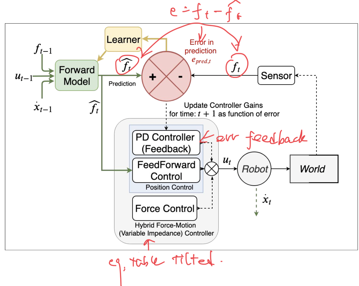
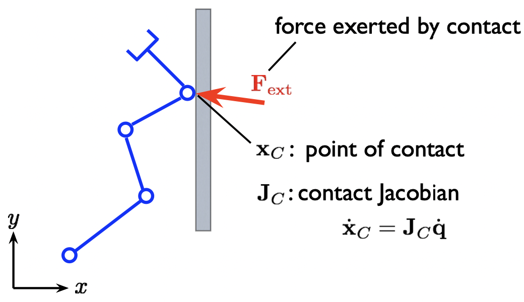
Impedance control

Robot with external forces $F_{ext}$, Inverse Dynamics: $M(q_d)\ddot{q}_d + C(q_d,\dot{q}_d)+G(q_d) = \tau \red- J^T_CF_{ext}$ Where sign is positive when force is applied BY robot, negetive when force is applied TO robot.

$J_C$ is the Jacobian for the point where external force is applied.

Impedance Control Equation: $M_d\ddot{\~x}+K_D\dot{\~x}+K_P\~x=F_{ext}$ Where $\ddot q=y-M^{-1}J^TF_{ext}$ $J\ddot q=\ddot x-\dot J\dot q$

$\~x = x_d-x$ $\ddot{x}=\dot J\dot q+Jy-JM^{-1}J^TF_{ext}$ $y=J^{-1}(\ddot{x}_d+M_d^{-1}K_D\dot{\~x}+M_d^{-1}K_P\~x-\dot J\dot q+\underbrace{M_d^{-1}F_{ext}+JM^{-1}J^TF_{ext}}_{\text{extra: force sensor at e.e.}})$

Hybrid Force-motion control

used for robot manipulator control
seperate control of force and motion
combine with impedance control of motion if necessary
provide compliance along some axes