FK/IK
Basics
- Degree of Freedom (DoF)
- Under-actuation
- Redundancy
- Workspace
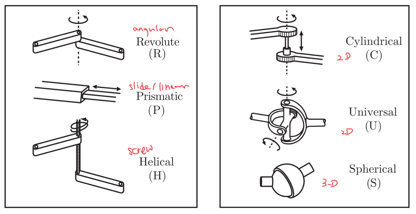
Typical robot joints 2 main type: Revolute & Prismatic
Robot configuration ( position of all points of the robot) Only focus on Rigidbody
End-effector configuration parameters: $X=\begin{bmatrix} X_P\ X_R \end{bmatrix}$
$X_P$: Position representations (3 DOF = 3 parameters)
- Cartesian $<x, y, z>$
- Cylindrical $<\rho, \theta, z>$
- Spherical $<r , \theta, \phi>$
$X_R$: Rotation Reps (3 DOF = 9 params - 6 constraints) $\leftarrow$ redundent expression
\(R = \begin{bmatrix} r_{11} & r_{12} & r_{13} \\ r_{21} & r_{22} & r_{23} \\ r_{31} & r_{32} & r_{33} \\ \end{bmatrix} = \begin{bmatrix} r_{1} & r_{2} & r_{3} \\ \end{bmatrix}\) Because the redundency in rotation matrix, so there MUST exist constraints (6) $ |r_1|=|r_2|=|r_3|=1 $
$ r_1\cdot r_2 = r_2\cdot r_3 = r_3\cdot r_1 = 0 $
angular representations:
- Euler Angles (
Z-Y-Z) - current frame - post multiplication - Euler ZYX Angles (Roll-Pitch-Yaw
Z-Y-X) - Fixed frame - left multiplication - Quaternions ( to avoid singularity )
From Rotation Matrix to Euler Angles
Use arc2
Q: What’s the properties of rotation matrix?
A:
- A rotation matrix will always be a square matrix.
- As a rotation matrix is always an orthogonal matrix
- the transpose will be equal to the inverse of the matrix.
- The determinant of a rotation matrix will always be equal to 1.
- Multiplication of rotation matrices will result in a rotation matrix.
- Furthermore, for clockwise rotation, a negative angle is used.
Q: how to determine a matrix is a rotation matrix. given $ R^A_B = \begin{bmatrix} \cos \theta & 0& \sin \theta
\sin \phi \sin\theta & \cos\phi & -\sin\phi\cos\theta
-\cos\phi\sin\theta & \sin\phi & \cos\phi\cos\theta
\end{bmatrix} $A: calculate the $det(R^A_B)=1$ and prove $R^{-1} = R^T \Leftrightarrow RR^T=I$
Degree of Freedon ( DOF )
homogeneous transformation
$~^A P$ is point P represented in coordinates A
$~^A_B T$ transform matrix from coordinates B to A
$ ~^A P = ~^A_B T ~^B P = ~^A_B T ~^B_C T ~^C P = ~^A_C T ~^C P $
$
\Rightarrow \red{~^A_C T = ~^A_B T ~^B_C T} =
\begin{bmatrix}
~^A_B R~^B_C R & ~^A_B R ~^B P_{origin C} + ~^A P_{origin B}
0^T & 1
\end{bmatrix}
$
Elementary Rotations
\(R_z(\alpha)= \begin{bmatrix} \cos \alpha & \red- \sin \alpha & 0\\ \sin \alpha & \cos \alpha & 0\\ 0 & 0 & 1\\ \end{bmatrix}\)
\[R_y(\beta)= \begin{bmatrix} \cos \beta & 0& \sin \beta \\ 0 & 1& 0\\ \red- \sin \beta & 0& \cos \beta \\ \end{bmatrix}\] \[R_x(\gamma)= \begin{bmatrix} 1 & 0& 0\\ 0 &\cos \gamma & \red- \sin \gamma \\ 0& \sin \gamma & \cos \gamma \\ \end{bmatrix}\]Rotate base on current frame => Post multiplication ( Right )
Rotate base on fixed frame => Pre multiplication ( Left )
Inverse
$ p^b=o^b_e+R_e^bp^e $
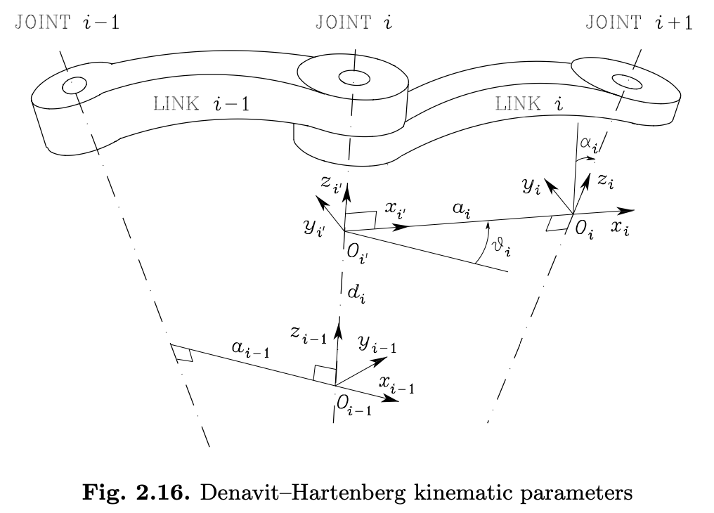
DH parameters (Denavit-Hartenberg)
P62 link
- z- prismatic translate along z; revolute rotate along z;
- Locate the origin Oi at the intersection of axis zi with the common normal to axes zi−1 and zi. Also, locate Oi′ at the intersection of the common normal with axis zi−1
- x- parallel to common normal of ( $z^{i-1}, z^i$), with direction from Joint i to Joint i + 1
- y- right hand coordinates
- di: distance between Oi-1 and Oi’ along zi-1
- θi: angle between xi-1 and xi about zi-1 (For revolute joints, θi defines the motion)
- ai: distance between Oi and Oi’
- $\alpha_i$: angle between zi-1 and zi about xi, positive for counter-clockwise.
(to make operation easier, try to define base frame overlap with 1st frame, & overlap intermediate frame)
- define z-
- origin ( intersection of common normal of $z^i, z^{i-1}$)
- $x^i$ is defined alone common normal, with direction of right hand from $z^{i-1}, z^i$
- y force right hand corrdinates
- $\alpha^i$ is right hand from $z^{i-1}, z^i$
- For Frame 0, only the direction of axis z0 is specified; then O0 and x0 can be arbitrarily chosen.
- For Frame n, since there is no Joint n + 1, zn is not uniquely defined while xn has to be normal to axis zn−1. Typically, Joint n is revolute, and thus zn is to be aligned with the direction of zn−1.
Homogeneous Transformation Matrix
Given the four D-H parameters for joint i: $a_i, d_i, \theta_i, \alpha_i$, we can compute the homogeneous transformation matrix from joint i-1 to joint i.
- choose a frame aligned with Frame i-1.
- Translate frame along $z_{i-1}$ by ${d_i}$ and rotate by $\theta_i$: \(A^{i-1}_{i'} = \begin{bmatrix} c\theta_i & -s\theta_i & 0 & 0 \\ s\theta_i & c\theta_i & 0 & 0 \\ 0 & 0 & 1 & d_i \\ 0 & 0 & 0 & 1\\ \end{bmatrix}\)
- Translate frame along $x_{i’}$ by $a_i$ and rotate by $\alpha_i$: \(A^{i'}_i = \begin{bmatrix} 1 & 0 & 0 & a_i \\ 0 & c\alpha_i & -s\alpha_i & 0 \\ 0 & s\alpha_i & c\alpha_i & 0 \\ 0 & 0 & 0 & 1\\ \end{bmatrix}\)
Resulting (Eq.2.52):
$
A^{i-1}i(q_i)=A^{i-1}{i’}A^{i’}_{i}=
\begin{bmatrix}
\pink{\cos\theta_i} & \pink{-\sin\theta_i}\cos\alpha_i & \sin\theta_i\sin\alpha_i & \pink{a_i\cos\theta_i}
\pink{\sin\theta_i} & \pink{\cos\theta_i}\cos\alpha_i & -\cos\theta_i\sin\alpha_i & \pink{a_i\sin\theta_i}
0 & \sin\alpha_i & \cos\alpha_i & d_i
0 & 0 & 0 & 1
\end{bmatrix}
$
For prismatic planar,
$
A^{i-1}_i(d_i)=
\begin{bmatrix}
1 & 0 & 0 & a_i
0 & \cos\alpha_i & -\sin\alpha_i & 0
0 & \sin\alpha_i & \cos\alpha_i & d_i
0 & 0 & 0 & 1
\end{bmatrix}
$
By computing each transformation from joint to joint, and post multiplying them all together, we have the complete transformation from the base frame to the end-effector frame
$
T^0_n(q)=A^0_1(q_1)A^1_2(q_2)…A^{n-1}_n(q_n) \
\Leftrightarrow X_e=k(q)=\begin{bmatrix}p_e & \phi_e\end{bmatrix}^T
$
$
q=\begin{bmatrix}q_1 & … & q_n\end{bmatrix}^T
$
where $q_i=\theta_i$ for revolute joint, $q_i=d_i$ for prismatic joint
Q: Given an arm, A:
- define frame
- define dh parameter
- computer post multiplication
Direct Kinematic Equation
\(x_e=k(q)\)
- k is a vector function that maps joint space($q=[q_1,q_2,q_n]^T$) to operational space([$P_x,P_y,P_z,R_x,R_y,R_z]^T$)
- k is the direct kinematics function
Note in general:
- k is a non-linear vector function
- k is surjective: every q vector gets mapped to one and only one xe vector.
- But not the other way around: k-1 is ill-posed: the number of solutions for k-1 may be zero, finite, or infinite
Jaccobian – w3
$
\frac{dx_e}{dt} =
\begin{bmatrix}
\frac{\partial k_1}{\partial q_1} & \frac{\partial k_1}{\partial q_2} & \frac{\partial k_1}{\partial q_3} \
\frac{\partial k_2}{\partial q_1} & \frac{\partial k_2}{\partial q_2} & \frac{\partial k_3}{\partial q_3}
\end{bmatrix}
\begin{bmatrix}
\frac{dq_1}{dt} \
\frac{dq_2}{dt} \
\frac{dq_3}{dt}
\end{bmatrix}
$
$ \Leftrightarrow \dot{X}_e=\pink{\frac{\partial k(q)}{\partial q}}\dot{q} = J(q)\dot{q} $
Q: Calculate the J of the arm.
A: $ X_e=\begin{bmatrix}p_x & p_y & \phi\end{bmatrix}^T=k(q)= \begin{bmatrix} a_1c_1+a_2c_{12}+a_3c_{123}
a_1s_1+a_2s_{12}+a_3s_{123}
\theta_1+\theta_2+\theta_3 \end{bmatrix} $ $J(q)=\frac{\partial k(q)}{\partial q} = \begin{bmatrix} -a_1s_1-a_2s_{12}-a_3s_{123} & -a_2s_{12}-a_3s_{123} & -a_3s_{123}
a_1c_1+a_2c_{12}+a_3c_{123} & a_2c_{12}+a_3c_{123} & a_3c_{123}
\theta_1 & \theta_2 & \theta_3 \end{bmatrix} $

Derive $J$
$ p^b=o^b_e+R_e^bp^e $ taking derivative on both side $\frac{d}{dt}p^b\Rightarrow$
\(\dot{p}^b=\overbrace{\dot{o}^b_e}^{\text{change in displacement between frames}}+\underbrace{\pink{\dot{R}^b_ep^e}}_{\text{velocity of rotation}}+\overbrace{R^b_e\dot{p}^e}^{\text{velocity w.r.t. end-eff frame }} \blue{\leftarrow\text{product rule}}\) where $\dot{R}^b_ep^e = \omega \times p^e_b = \omega \times R^b_ep^e$
$ \omega_i=\omega_{i-1}+\pink{\omega_{i-1,i}} \blue{\leftarrow \text{relative rotation between 2 frames}} $
Singularities / Redundancy
When J drops ranks, not inversible. Calculate $det(J) =0$
Rank: number of linearly independent columns = number of linearly independent rows = number of DOFs in the Range space
#DOFs in operational space + #DOFs in null space = #DOFs of the robot (n)
Ways to deal with singularities:
- try to stay away from them
- change task priorities
- use damped least squares
- Jacobian Transpose (numerically very simple! but need to assume: $\dot x_ d = 0$ )
Inverse Kinematics
\(\dot q = J^+ \dot x + \underbrace{( I - J ^+ J ) }_{\text{null space projection matrix}}\dot q_0\) where $J^+ = J^T (JJ^T )^{-1}$ is Moore-Penrose pseudoinverse.
$\dot q_0$ can be used to achieve secondary objectives.