Home > Robot Vision > CV

THANKS @mantasu for Notes

Visual Perception

Computational Vision

Computational Vision - the process of discovering from images what is present in the world and where. It is challenging because it tries to recover lost information when reversing the imaging process (imperfect imaging prcess, discretized continuous world)

Applications:

Automated navigation with obstacle avoidance
Scene recognition and target detection
Document processing
Human computer interfaces

Human Vision

Captured photons release energy which is used as electrical signals for us to see. Pupils dilate to accept as much light as needed to see clearly. Rod cells (~120m) are responsible for vision at low light leves, cones (~6m) are active at higher levels and are capable of color vision and have high spacial acuity. There’s a 1-1 relationship of cones and neurons so we are abe to resolve better, meanwhile many rods converge to one neuron.

Receptive field - area on which light must fall for neuron to be stimulated. A receptive field of a Ganglion cell is formed from all photoreceptors that synapse with it.

Ganglion cells - cells located in retina that process visual information that begins as light entering the eye and transmit it to the brain. There are 2 types of them.

On-center - fire when light is on centre
Off-center - fire when light is around centre

Ganglion cells allow transmition of information about contrast. The size of the receptive field controls the spatial frequency information (e.g., small ones are stimulated by high frequencies for fine detail). Ganglion cells don’t work binary (fire/not fire), the change the firing rate when there’s light.

Trichromatic coding - any color can be reproduced using 3 primary colors (red, blue, green).

Retina contains only 8% of blue cones and equal proportion of red and green ones - they allow to discriminate colors 2nm in difference and allow to match multiple wavelengths to a single color (does not include blending though)

Maths

Wave frequency $f$ (Hz) and energy $E$ (J) can be calculated as follows ($h=6.623\times 10^{34}$ - Plank’s constant, $c=2.998\times 10^8$ - speed of light):

\[\text{frequency}(Hz) \rightarrow f=\frac{c \leftarrow \text{speed of light} (2.998*10^8 ms^{-1}) }{\lambda \leftarrow \text{wavelength}(m)}\] \[E=hf\]

Human erceivable electromagnetic radiation wavelengths are within 380 to 760 nm

Law of Geometric Optics:

Light travels in straight lines
Ray, its reflection and the normal are coplanar
Ray is refracted when it transits medium

Snell’s Law - given refraction indeces $n_1$ and $n_2$, and “in” and “out” angles $\alpha_1$ and $\alpha_2$, there is a relation: $n_1 \sin \alpha_1=n_2 \sin \alpha_2$

Focal length $f$ (m) - distance from lens to the point $F$ where the system converges the light. The power of lens (how much the lens reduces the real world to the image in plane) is just $\frac{1}{f}$ (D) (~59D for human eye). For concave lens: $\frac{1}{f}=\frac{1}{u}+\frac{1}{v}$

Lens Formula and Magnification

If the image plane is curved (e.g., back of an eye), then as the angle from optical center to real world object $\tan\theta=\frac{h}{u}=\frac{h’}{v}$ gets larger (when it gets closer to the lens), it is approximated worse.

Edge Detection and Filters

Edge Detection

Intensity image - a matrix whose values correspond to pixels with intensities within some range. (imagesc in matlab displays intensity image).

Colormap - a matrix which maps every pixel to usually (most popular are RGB maps) 3 values to represent a single color. They’re averaged to convert it to intensity value.

Image - a function $f(x, y)$ mapping coordinates to intensity. We care about the rate of change in intensity in x and y directions - this is captured by the gradien of intensity Jacobian vector:

\[\nabla f(x, y)=\begin{pmatrix}{\partial f} / {\partial x} \\ {\partial f} / {\partial y}\end{pmatrix}\]

Such gradient has x and y component, thus it has magnitude and direction:

\[M(\nabla f)=\sqrt{(\nabla_xf)^2+(\nabla_yf)^2}\] \[\alpha=\tan^{-1}\left(\frac{\nabla_yf}{\nabla_xf}\right)\]

Edge detection is useful for feature extraction for recognition algorithms

Detection Process

Edge dectiptors:

Edge direction - perpendicular to the direction of the highest change in intensity (to edge normal)
Edge strength - contrast along the normal
Edge position - image position where the edge is located

Edge detection steps:

Smoothening - remove noise
Enhancement - apply differentiation
Thresholding - determine how intense are edges
Localization - determine edge location

Optimal edge detection criteria:

Detecting - minimize false positives and false negatives
Localizing - detected edges should be close to true edges
Single responding - minimize local maxima around the true edge

First order Edge Filters

To approximate the gradient at the center point of 2-by-2 pixel area, for change in x - we sum the differences between values in rows; for change in y - the differences between column values. We can achieve the same by summing weighted pixels with horizontal and vertical weight matrices (by applying cross-correlation):

\[W_x=\begin{bmatrix}-1 & 1 \\ -1 & 1\end{bmatrix};\ W_y=\begin{bmatrix}1 & -1 \\ 1 & -1\end{bmatrix}\]

There are other ways to approximate the gradient (not necessarily at 2-by-2 regions): Roberts and Sobel (very popular):

\[W_x=\begin{bmatrix}1 & 0 \\ 0 & -1\end{bmatrix};\ W_y=\begin{bmatrix}0 & -1 \\ 1 & 0\end{bmatrix}\] \[W_x=\begin{bmatrix}-1 & 0 & 1 \\ -2 & 0 & 2 \\ -1 & 0 & 1\end{bmatrix};\ W_y=\begin{bmatrix}1 & 2 & 1 \\ 0 & 0 & 0 \\ -1 & -2 & -1\end{bmatrix}\]

After applying filters to compute the gradient matrices $G_x$ and $G_y$, we can calculate the magnitude between the 2 to get the final output: $M=\sqrt{G_x^2 + G_y^2}$. Sometimes it’s approximated by magnitude values.

Note that given an intensity image $I$ of dimensions $H\times W$ and a filter (kernel) $K$ of dimensions $(2N+1)\times (2M+1)$ the cross-correlation at pixel $h, w$ is expressed as (odd-by-odd filters are more common as we can superimpose the maps onto the original images we want to compare):

\[(I\otimes K)_{h,w}=\sum_{n=-N}^N\sum_{m=-M}^MI_{h+n,w+m}K_{N+n,M+m}\]

We usually set a threshold for calculated gradient map to distinguish where the edge is.

If we use noise smoothing filter, instead of looking for an image gradient after applying the noise filter, we can take the derivative of the noise filter and then convolve it (because mathematically it’s the same):

\[\nabla_x(h\star f)=(\nabla_xh)\star f\]

Second order Edge Filters

We can apply Laplacian Operator - by applying the second derivative we can identify where the rate of change in intensity crosses 0, which shows exact edge.

Laplacian - sum of second order derivatives (dot product):

\[\nabla f=\nabla^2 f=\nabla \cdot \nabla f\] \[\nabla^2I=\frac{\partial^2I}{\partial x^2}+\frac{\partial^2I}{\partial y^2}\]

For a finite difference approximation, we need a filter that is at least the size of 3-by-3. For change in x, we take the difference between the differences involving the center and adjacent pixels for that row, for change in y - involving center and adjacent pixels in that column. I. e., in 3-by-3 case:

\[(\nabla_{x^2}^2I)_{h,w}=(I_{h,w+1}-I_{h,w}) - (I_{h,w} - I_{h,w-1})=I_{h,w-1}-2I_{h,w}+I_{h,w+1}\] \[(\nabla_{y^2}^2I)_{h,w}=I_{h-1,w}-2I_{h,w}+I_{h+1,w}\]

We just add the double derivative matrices together to get a final output. Again, we can calculate weights for these easily to represent the whole process as a cross-correlation (a more popular one is the one that accounts for diagonal edges):

\[W=\begin{bmatrix}0 & 1 & 0 \\ 1 & -4 & 1 \\ 0 & 1 & 0\end{bmatrix};\ W=\begin{bmatrix}1 & 4 & 1 \\ 4 & -20 & 4 \\ 1 & 4 & 1\end{bmatrix}\]

Noise Removal

We use a uniform filter (e.g., in 3-by-3 case all filter values are $\frac{1}{9}$) to average random noise - the bigger the filter, the more details we lose but the less noise the image has due to its smoothness. More popular filters are Gaussian filters with more weight on middle points. Gaussian filter can be generated as follows:

\[H_{ij}= \frac{1}{2\pi\sigma^2}\exp \left(-\frac{(i-(k+1))^2+(j-(k+1))^2}{2\sigma^2} \right) ; 1 \leq i, j \leq (2k + 1)\]

Laplacian of Gaussian - Laplacian + Gaussian which smoothens the image (necessary before Laplacian operation) with Gaussian filter and calculates the edge with Laplacian Operator

Note the noise suppression-localization tradeoff: larger mask size reduces noise but adds uncertainty to edge location. Also note that the smoothness for Gaussian filters depends on $\sigma$.

Canny Edge Detector

Canny has shown that the first derivative of the Gaussian provides an operator that optimizes signal-to-noise ratio and localization

Algorithm:

Compute the image gradients $\nabla_x f = f * \nabla_xG$ and $\nabla_y f = f * \nabla_yG$ where $G$ is the Gaussian function of which the kernels can be found by:
- $\nabla_xG(x, y)=-\frac{x}{\sigma^2}G(x, y)$
- $\nabla_yG(x, y)=-\frac{y}{\sigma^2}G(x, y)$
Compute image gradient magnitude and direction
Apply non-maxima suppression
Apply hysteresis thresholding

Non-maxima suppression - checking if gradient magnitude at a pixel location along the gradient direction (edge normal) is local maximum and setting to 0 if it is not

Hysteresis thresholding - a method that uses 2 threshold values, one for certain edges and one for certain non-edges (usually $t_h = 2t_l$). Any value that falls in between is considered as an edge if neighboring pixels are a strong edge.

For edge linking high thresholding is used to start curves and low to continue them. Edge direction is also utilized.

Scale Invariant Feature Transform

SIFT - an algorithm to detect and match the local features in images

Invariance Types (and how to achieve them):

Illumination - luminosity changes
- Difference based metrics
Scale - image size change
- Pyramids - average pooling with stride 2 multiple times
- Scale Space - apply Pyramids but take DOGs (Differences of Gaussians) in between and keep features that are repeatedly persistent
Rotation - roll the image along the x axis
- Rotate to most dominant gradient direction (found by histograms)
Affine -
Perspective -

Motion

Visual Dynamics

By analyzing motion in the images, we look at part of the anatomy and see how it changes from subject to subject (e.g., through treatment). This can also be applied to tracking (e.g., monitor where people walk).

Optical flow - measurement of motion (direction and speed) at every pixel between 2 images to see how they change over time. Used in video mosaics (matching features between frames) and video compression (storing only moving information)

There are 4 options of dynamic nature of the vision:

Static camera, static objects
Static camera, moving objects
Moving camera, static objects
Moving camera, moving objects

Difference Picture - a simplistic approach for identifying a feature in the image $F(x, y, i)$ at time $i$ as moved:

\[DP_{12}(x,y)=\begin{cases}1 & \text{if }\ |F(x,y,1)-F(x,y,2)|>\tau \\ 0 & \text{otherwise}\end{cases}\]

We also need to clean up the noise - pixels that are not part of a larger image . We use connectedness (more info at 1:05):

2 pixels are both called 4-neighbors if they share an edge
2 pixels are both called 8-neighbors if they share an edge or a corner
2 pixels are 4-connected if a path of 4-neighbors can be created from one to another
2 pixels are 8-connected if a path of 8-neighbors can be created from one to another

Motion Correspondence

Aperture problem - a pattern which appears to be moving in one direction but could be moving in other directions due to only seeing the local features movement. To solve this, we use Motion Correspondence (matching).

Motion Correspondence - finding a set of interesting features and matching them from one image to another (guided by 3 principles/measures):

Discreteness - distinctiveness of individual points (easily identifiable features)
Similarity - how closely 2 points resemble one another (nearby features also have similar motion)
Consistency - how well a match conforms with other matches (moving points have a consistent motion measured by similarity)

Most popular features are corners, detected by Moravec Operator (paper) (doesn’t work on small objects). A mask is placed over a region and moved in 8 directions to calculate intensity changes (with the biggest changes indicating a potential corner)

Algorithm of Motion Correspondence:

Pair one image’s points of interest with another image’s within some distance
Calculate degree of similarity for each match and the likelihood
Revise likelihood using nearby matches

Degree of similarity $s$ is just the sum of squared differences of pixels between 2 patches $i$ and $j$ (of size $N\times N$) and the likelihood is just the normalized weights $w$ (where $\alpha$ - constant) $s_{ij}=\sum_{n=1}^{N\times N}(p_i^{(n)}-p_j^{(n)})^2$ $w_{ij}=\frac{1}{1+\alpha s_{ij}}$

Hough Transform

A point can be represented as a coordinate (Cartesian space) or as a point from the origin at some angle (Polar space). It has many lines going through and each line can be described as a vector by angle and magnitude $w$ from some origin:

\[w=x \cos \theta + y \sin \theta\]

Hough Space - a plane defined by $w$ and $\theta$ which takes points $(x, y)$ in image space and represents them as sinusoids in the new space. Each point in such space $(w, \theta)$ is parameters for a line in the image space.

Hough Transform - picking the “most voted” intersections of lines in the Hough Space which represent line in the image space passing through the original points (sinusoids in Hough Space)

Algorithm:

Create $\theta$ and $w$ for all possible lines and initialize 0-matrix $A$ indexed by $\theta$ and $w$
For each point $(x, y)$ and its every angle $\theta$ calculate $w$ and add vote at $A[\theta, w]+=1$
Return a line where $A>\text{Threshold}$

There are generalized versions for ellipses, circles etc. (change equation $w$). We also still need to suppress non-local maxima

Image Registration & Segmentation

Registration

Image Registration - geometric and photometric alignment of one image to another. It is a process of estimating an optimal transformation between 2 images.

Image registration cases:

Individual - align new with past image (e.g, rash and no rash) for progress inspection; align similar sort images (e.g., MRI and CT) for data fusion.
Groups - many-to-many alignment (e.g., patients and normals) for statistical variation; many-to-one alignment (e.g., thousands of subjects with different sorts) for data fusion

Image Registration problem can be expressed as finding transformation $T$ (i.e., parameterized by $\mathbf{p}$) which minimizes the difference between reference image $I$ and target image $J$ (i.e., image after transformation):

\[\mathbf{p}^*=\operatorname*{argmin}_\mathbf{p} \sum_{k=1}^K\underbrace{\text{sim}\left(I(x_k), J(T_{\mathbf{p}}(x_k))\right)}_}\]

Components of Registration

Entities to match

We may want to match landmarks (control points), pixel values, feature maps or a mix of those.

Type of transform

Transformations include affine, rigid, spline etc. Most popular:

Rigid - composed of 3 rotations and 3 translations (so no distortion). Transforms are linear and can be a 4x4 matrices (1 translation and 3 rotation).
Affine - composed of 3 rotations, 3 translations, 3 stretches and 3 shears. Transforms are also linear and can be represented as 4x4 matrices
Piecewise Affine - same as affine except applied to different components (local zones) of the image, i.e., a piecewise transform of 2 images.
Non-rigid (Elastic) - transforming via 2 forces - external (deformation) and internal (constraints) - every pixel moves by different amount (non-linear).

Similarity function

Conservation of Intensity - pixel-wise MSE/SSD. If resolution is different, we have to interpolate missing values which results in poor similarity

\[\text{MSE}=\frac{1}{K}\sum_{k=1}^K \left(I(x_k) - J(T_{\mathbf{p}}(x_k))\right)^2\]

Mutual Information - maximize the clustering of the Joint Histogram (maximize information which is mutual between 2 images):

Image Histogram (hist) - a normalized histogram (y - num pixels, x - intensity) representing a discrete PDF where peaks represent some regions.
Joint Histogram (histogram2) - same as histogram, expcept pairs of intensities are counted (x, y - intensities, color - num pixel pairs). Sharp heatmap = high similarity.

\[\text{MI}(I,J|T)=\sum_{i\in I}\sum_{j\in J}p(i,j)\log\frac{p(i,j)}{p(i) p(j)}\]

Where $p(i)$ - probability of intensity value $i$ (from image histogram)

Normalized Cross-Correlation - assumes there is a linear relationship between intensity values in the image - the similarity measure is the coefficient ($\bar A$ and $\bar B$ - mean intensity values):

\[CC=\frac{1}{N}\frac{\sum_{i\in I}(A(i)-\bar A)(B(i)-\bar B)}{\sqrt{\sum_{i\in I}(A(i)-\bar A)^2\sum_{i\in I}(A(i)-\bar A)^2}}\] \[CC=\frac{\text{Cov}[A(i), B(i)]}{\sigma[A(i)]\sigma[B(i)]}\]

More details: correlation, normalized correlation, correlation coefficient, covariance vs correlation, correlation as a similarity measure

Segmentation

Image Segmentation - partitioning image to its meaningful regions (e.g., based on measurements on brightness, color, motion etc.). Non-automated segmentation (by hand) require expertise; Automated segmentation (by models) are currently researched

Image representation:

Dimensionality: 2D (x, y), 3D (x, y, z), 3D (x, y, t), ND (x, y, z, b2, …, bn)
Resolution: spatial (pixels/inch), intensity (bits/pixel), time (FPS), spectral (bandwidth)

Image characterization:

As signals: e.g., frequency distribution, signal-to-noise-ratio
As objects: e.g., individual cells, parts of anatomy

Segmentation techniques

Region-based: global (single pixels - thresholding), local (pixel groups - clustering)
Boundary-based: gradients (finding contour energy), models (matching shape boundaries)

Semi-Automated Segmentation

Thresholding

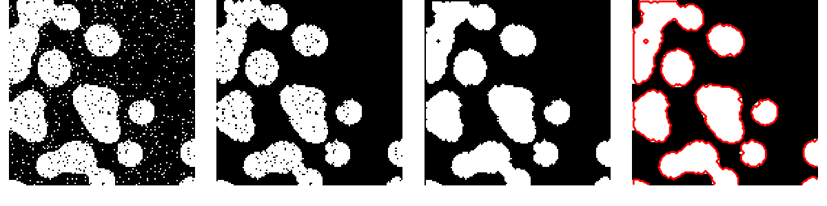
Thresholding - classifying pixels to “objects” or “background” depending on a threshold $T$ which can be selected from image histogram dips. If the image is noisy, threshold can be interactive (based on visuals), adaptive (based on local features), Otsu

Otsu threshold - calculating variance between 2 objects for exhaustive number of thresholds and selecting the one that maximizes inter-class intensity variance (biggest variation for 2 different objects and minimal variation for 1 object)

Smoothing the image before selecting the threshold also works. Mathematical Morphology techniques can be used to clean up the output of thresholding.

Mathematical Morphology

Mathematical Morphology (MM) - technique for the analysis and processing of geometrical structures, mainly based on set theory and topology. It’s based on 2 operations - dilation (adding pixels to objects) and erosion (removing pixels from objects).

An operation of MM deals with large set of points (image) and a small set (structuring element). A structuring element is applied as a convolution to touch up the image based on its form.

Applying dilation and erosion multiple times lets to close the holes in segments

Mathematical Morphology

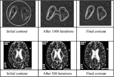
Active Contours

Active Contours - energy minimization problem where we want to find the equilibrium (lowest potential) of the three terms:

$(E_{int})$ Internal - sensitivity to the amount of stretch in the curve (smoothness along the curve)
$(E_{img})$ Image - correspondence to the desired image features, e.g., gradients, edges, colors
$(E_{ext})$ External - user defined constraints/prior knowledge over the image structure (e.g., starting region)

\[E[C(p)]=\alpha \int_0^1 E_{int}[C(p)]dp + \beta \int_0^1 E_{img}[C(p)]dp + \gamma \int_0^1 E_{ext}[C(p)]dp\]

Energy in the image is some function of the image features; Snake is the object boundary or contour

Watershed

Watershed Segmentation - classifying pixels to 3 classes based on thresholding: local minima (min value of a region), catchment basin (object region), watershed (object boundary)

Face Recognition with PCA

PCA

PCA - algorithm that determines the dominant modes of variation of the data and projects the data onto the coordinate system matching the shape of the data.

Covariance - measures how much each of the dimensions vary with respect to each other. Given a dataset $D={\mathbf{x_1},…,\mathbf{x_N}}$, where $\mathbf{x_N}\in\mathbb{R}^{D}$, the variance of some feature in dimension $i$ and the covariance between a feature in dimension $i$ and a feature in dimension $j$ can be calculated as follows:

\[Var[x_i]=E[(x_i-E[\mathbf{x}_i])^{2}]\] \[Cov[x_i, x_j]=\Sigma_{x_i, x_j}=E[(x_i - E[\mathbf{x}_i])(x_j - E[\mathbf{x}_j])]\]

Covariance matrix has variances on the diagonal and cross-covariances on the off-diagonal. If cross-covariances are 0s, then neither of the dimensions depend on each other. Given a dataset $D={\mathbf{x_1},…,\mathbf{x_N}}$, where $\mathbf{x_N}\in\mathbb{R}^{D}$, the dataset covariance matrix can be calculated as follows:

\[Var[D]=\Sigma=\frac{1}{N}\sum_{n=1}^N(\mathbf{x}_i-E[D])(\mathbf{x}_i-E[D])^{\top}=(D-E[D])(D-E[D])^{\top}\]

Identical variance - the spread for every dimension is the same
Identical covariance - the correlation of different dimensions is the same

PCA chooses such $d^{th}$ columns for $W$ that maximize the variances of projected (mean subtracted) vectors and are orthogonal to each other (meaning information is completely different).

\[\tilde Y = Y - \bar Y\] \[Var[\tilde Y \mathbf{w}]=(\tilde Y\mathbf{w})^{\top}\tilde Y \mathbf{w}=\mathbf{w}^{\top}\Sigma\mathbf{w}\]

PCA thus becomes an optimization problem constrained to $\mathbf{w}^{\top}\mathbf{w}=\mathbf{1}$ (so that the norm would not go to infinity). Finding the gradient and setting it to 0 shows that the columns of $W$ are basically eigenvectors of the covariance matrix $\Sigma$ of high dimensional space $Y$.

\[\mathcal{F}=\arg\max_{\mathbf{w}}(\mathbf{w}^{\top}\Sigma\mathbf{w} - \lambda(\mathbf{w}^{\top}\mathbf{w}-\mathbf{1}))\] \[\Sigma\mathbf{w}=\lambda\mathbf{w}\]

In general, the optimization solution for covariance matrix $\Sigma$ will provide $M$ eigenvectors $\begin{bmatrix}\mathbf{w}1 & \cdots & \mathbf{w}_M\end{bmatrix}$ and $M$ _eigenvalues $\begin{bmatrix}\lambda_1 & \cdots & \lambda_M\end{bmatrix}$. The eigenvectors are the principal components of $Y$ ordered by eigenvalues.

PCA works well for linear transformation however it is not suitable for non-linear transformation as it cannot change the shape of the datapoints, just rotate them.

Singular Value Decomposition - a representation of any $X\in\mathbb{R}^{M\times N}$ matrix in terms of the product of 3 matrices:

\[X=UDV^{\top}\]

Where:

$U\in\mathbb{R}^{M\times M}$ - has orthonormal columns (eigenvectors)
$V\in\mathbb{R}^{N\times N}$ - has orthonormal columns (eigenvectors)
$D\in\mathbb{R}^{M\times N}$ - diagonal matrix and has singular values of $X$ on its diagonals ($s_1>s_2>…>0$) (eigenvalues)

In the case of images $\Sigma$ would be $N\times N$ matrix where $N$ - the number of pixles (e.g., $256\times 256=65536$). It could be very large therefore we don’t explicitly compute covariance matrix.

Face Recognition

Eigenface - a basis face which is used within a weighted combination to produce an overall face (represented by x - eigenface indices and y - eigenvalues (weights)). They are stored and can be used for recognition (not detection!) and reconstruction.

Face representation

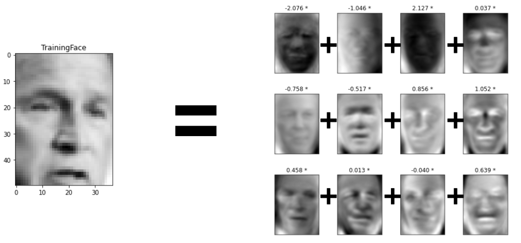
To compute eigenfaces, all face images are flattened and rearranged as a 2D matrix (rows = images, columns = pixels). Then the covariance matrix and its eigenvalues are found which represent the eigenfaces. Larger eigenvalue = more distinguishing.

Recognition

To map image space to “face” space, every image $\mathbf{x}i$ is multiplied by every _eigenface $\mathbf{v}_k$ to get a respective set of weights $\mathbf{w}_i$:

\[\mathbf{w}_i=\begin{bmatrix}(\mathbf{x}_i-\bar{\mathbf{x}})^{\top}\mathbf{v}_1 & \cdots & (\mathbf{x}_i-\bar{\mathbf{x}})^{\top}\mathbf{v}_K\end{bmatrix}^{\top}\]

Given a weight vector of some new face $\mathbf{w}{\text{new}}$, it is compared with every other vector based on _euclidean distance $d$:

\[d(\mathbf{w}_{\text{new}}, \mathbf{w}_{i})=||\mathbf{w}_{\text{new}} - \mathbf{w}_{i}||_2\]

Note that the data must be comparable (same resolution) and size must be reasonable for computational reasons

Medical Image Analysis

Ultraviolet Techniques

Thermography - imaging of the heat being radiated from an object which is measured by infrared cameras/sensors. It helps to spot increased blood flow and metabolic activity when there is an inflammation (detects breast cancer, ear infection).

X-Ray

Process of taking an x-ray photo: A lamp generates electrons which are bombarded at a metal target which in turn generates high energy photons (x-rays). They go though some medium (e.g., chest) and those which pass though are captured on the other side what results in a black

white image (e.g., high density (bones) = white, low density (lungs) = black)

X-ray photos are good to determine structure but we cannot inspect depth

Computed Tomography (CT)

Process of 3D reconstruction via computed tomography (CT): An x-ray source is used to perform multiple scans across the medium to get multiple projections. The data is then back-projected to where the x-rays travelled to get a 3D representation of a medium. In practice filtered back-projections are used with smoothened (convolved with a filter) projected data.

CT reconstructions are also concerned with structural imaging

Nuclear Medical Imaging

Process of nuclear medical imaging via photon emission tomography (PET): A subject is injected with radioactive tracers (molecules which emit radioactive energy) and then gamma cameras are used to measure how much radiation comes out of the body. The detect the position of each gamma ray and back-projection again is used to reconstruct the medium.

Nuclear Imaging is concerned with functional imaging and inspects the areas of activity. However, gamma rays are absorbed in different amounts by different tissues, therefore, it is usually combined with CT

X-Ray Scans

CT Scan Process

PET Scan Process

Other Techniques

Ultrasound Imaging

Ultrasound - a very high pitched sound which can be emitted to determine location (e.g., by bats, dolphins). Sonar devices emit a high pitch sound, listen for the echo and determine the distance to an object based on the speed of sound.

Process of ultrasound imaging using ultrasound probes: An ultrasound is emitted into a biological tissue and the reflection timing is detected (different across different tissue densities) which helps to work out the structure of that tissue and reconstruct its image.

The resolution of ultrasound images is poor but the technique is harmless to human body

Light Imaging

Process of light imaging using pulse oximeters: as blood volume on every pulse increases, the absorption of red light increases so the changes of the intensity of light can be measured through time. More precisely, the absorption at 2 different wavelengths (red and infrared) corresponding to 2 different blood cases (oxy and deoxy) is measured whose ratio helps to infer the oxygen level in blood.

Tissue scattering - diffusion and scattering of light due to soft body. This is a problem because it produces diffused imaging (can’t determine from which medium light bounces off exactly (path information is lost), so can’t do back-projection)

Several ways to solve tissue scattering:

Multi-wavelength measurements and scattering change detection - gives information on how to resolve the bouncing off
Time of flight measurements (e.g., by pulses, amplitude changes) - gives information on how far photons have travelled

Process of optical functional brain imaging using a light detector with many fibers: A light travels through skin and bone to reach the surface of the brain. While a subject watches a rotating checkerboard pattern, an optical signal in the brain is measured. Using a 3D camera image registration, brain activity captured via light scans can be reconstructed on a brain model.

Magnetic Resonance Imaging (MRI)

Process of looking at water concentration using magnetic devices: A subject is put inside a big magnet which causes spinning electrons to align with magnetic waves. Then a coil is used around the area of interest (e.g., a knee) which uses radiofrequency - it emits a signal which disrupts the spinning electrons and collects the signal (the rate of it) emitted when the electrons come back to their axes. Such information is used to reconstruct maps of water concentration.

Functional MRI (FMRI) - due to oxygenated blood being more magnetic than deoxygenated blood, blood delivery can be monitored at different parts of the brain based on when they are activated (require oxygenated blood).

MRI is structural and better than CT because it gives better contrast between the soft tissue

Ultrasound imaging

Pulse oximeter

MRI Scanner

Object Recognition

Model Based

Viewpoint-invariant - non-changing features that can be obtained regardless of the viewing conditions. More sensitivity requires more features which is challenging to extract and more stability requires fewer features which are always constant.

Marr’s model-based approach on reconstructing 3D scene from 2D information:

Primal sketch - understanding what the intensity changes in the image represent (e.g., color, corners)
2.5D sketch - building a viewer-centered representation of the object (object can be recognized from viewer angle)
Model selection - building an object-centered representation of the object (object can be recognized from all angles)

Marr’s algorithm approaches the problem in a top-down approach (like brain): it observes a general shape (e.g., human), and then if it needs it gets into details (e.g., every human hair). It’s object-centered - shape doesn’t change depending on view.

Recognition by Components Theory - recognizing objects by matching visual input against structural representations of objects in the brain, consisting of geons and their relations

The problem is that there is an infinite variety of objects so there is no efficient way to represent and store the models of every object. Even a library containing 3D parts (building blocks), would not be big enough and would need to be generalized.

Appearance Based

Appearance based recognition - characterization of some aspects of the image via statistical methods. Useful when a lot of information is captured using multiple viewpoints because An object can look different from a different angle and it may be difficult to recognize using a model which is viewpoint-invariant. A lot of processing is involved in statistical approach.

SIFT can be applied to find features in the desired image which can further be re-described (e.g., scaled, rotated) to match the features in the dataset for recognition (note: features must be collected from different viewpoints in the dataset)

Category Level Recognition

Part Based Model - identifying an object by parts - given a bag of features within the appearance model, the image is checked for those features and determined whether it contains the object. However, we want structure of the parts (e.g., order)

Constellation Model - takes into account geometrical representation of the identified parts based on connectivity models. It is a probabilistic model representing a class by a set of parts under some geometric constraints. Prone to missing parts.

Hierarchical Architecture for object recognition (extract to hypothesize, register to verify):

Extract local features and learn more complex compositions
Select the most statistically significant compositions
Find the category-specific general parts

Appearance based recognition is a more sophisticated technique as it is more general for different viewpoints, however model based techniques work well for non-complex problems because they are very simple.