Unsupervised Learning
Labelled data is limited (time consuming, requires expertise, label in every possible situation).
Unsupervised learning: From observations ($X$) to latent variables ($Z$, infer), without labeled data.
Available data: $x_1, …, x_N \sim \mathcal{p}_{data}(x)$
Goal: Learn useful features of the data / Learn the structure of the data.
Used for:
- Represent data to a lower dimension through PCA (compress image or audio)
- Group data by similarity through clustering (text analysis, social media users, produce labelled data)
- Estimate PDF through Probability Density Estimation (generate fake data)
- Create style or fake images through generation / synthesise (synthesize shoe styles from contours just by giving a few examples, image enhancement)
Auto-Encoders
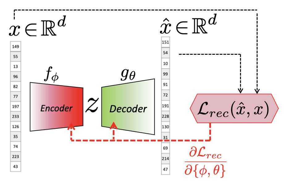
Given data we want the model to infer something about the content/characteristics, i.e., the latent variable. We encode the data first, then decode it. We use bottleneck layer in the middle to compress the data we’re learning (otherwise, if it’s of the same dimension, the parameters would only be the identity matrices)
Standard / Basic AE refers to AE with bottleneck
Reconstruction error - in most cases just MSE(Mean-Squared Error) which includes the parameters of the encoder $f_{\phi}$ and the decoder $g_{\theta}$. We minimize it to 0 when finding optimal parameters.
Compression forces the encoder to learn the most prominent features
Trade-off: Wider-bottleneck structure gives better construction & less compression.
Applications:
- Compress data - and encoded movie could be stored on a server, a decoder could be stored on a cloud or user’s computer which would allow fast streaming with reduced resources
- Cluster data - encoders in a way cluster data due to the same decoder - it has to cluster latent variables if it wants to recreate similar representations for similar input data
- Learn a classifier - we keep the encoder that produces cluster representation (tho not necessarily useful for classifier) and attach a classifier that learns the decision boundaries
- Data synthesis - we keep the decoder and sampling a random latent variable (if it is within realistic space). Due to curse of dimensionality, vanilla AEs are NOT appropriate for this because a randomly sampled latent variable in high dimension can be sampled from an unrepresentative space (i.e., where no real data would be encoded to)
NOT trained for generate new fake data. -> sampling problems, gaps in input space.
Generative Model
“A generative model describes how a dataset is generated, in terms of a probabilistic model. By sampling from this model, we are able to generate new data.” –Generative Deep Learning, David Foster
We train them to perform probability density estimation
For frequency-based approximation techniques the number of samples needed to fill the space grows exponentially with the number of dimensions.
In high dimensions, the input space would basically be empty. => So difficult to do PDE directly. => Indirectly by enforcing samples from model to be similar to real data. (VAEs / GANs)
Variational Auto-Encoders
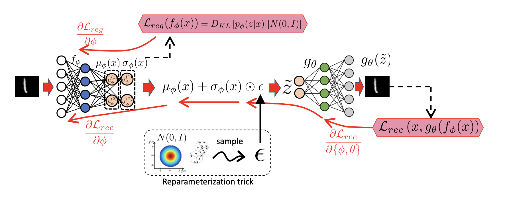
VAE - uses an encoder that maps each input to a small multivariate Gaussian (with uncorrelated dimensions) which is part of a larger prior distribution and a decoder which is forced to decode from that prior
\[p_{\phi}(\mathbf{z}|\mathbf{x})=\mathcal{N}(\bm \mu_{\phi}(\mathbf{x}), \bm \sigma_{\phi}(\mathbf{x})^2)\]Note: because standard deviation must be positive, we assume the raw output of an encoder is log of standard deviation $\log (\bm \sigma_{\phi}(\mathbf{x}))$. To get actually get it, we apply the exponent. Not using ReLU due to bad gradient around
0thus neurons die quickly.
Stochastic Decoder - decoder which at each SGD iteration for each input draws a different encoded sample that is determined by the probability clusters and tries to reconstruct any sample, even the unlikely ones.
Overall loss function for VAE consists of 2 parts. Reconstruction loss helps to learn to create new realistic data and the regularizer takes care of the prior. We want to minimize the loss on average over all training data.
| With reconstruction loss, we try to reproduce $x$ for any $\tilde z \sim p_{\phi}(z | x)$ as opposed to directly encoded point $f_{\phi}(x)$. If Gaussians overlap, the loss is high. It learns means that cluster samples and small STDs that reduce overlap. |
With regularization we prevent distributions to turn to points (with 0 std) - we minimize KL Divergence between predicted posterior $\tilde z$ and Gaussian $\mathcal{N}(0, I)$. $D_{KL}$ between 2 Gaussians. Causes means to be around 0 and STDs to cover prior.
Re-parameterization - since sampling is not differentiable, we give a constant to the network $\epsilon \sim \mathcal{N}(0, I)$ with which it simulates sampling $\tilde z=\mu_{\phi}(x)+\sigma_{\phi}\odot \epsilon$.
Applications:
- Generation - synthesizing new data. Note that in space of $\tilde Z$ there may still be gaps due to small $\lambda$ encouraging separation of dissimilar data and because SGD may end up in local optimum.
- Interpolation - given some $\tilde z$, move from obe to another and see what values get produced. They’re a lot smoother with VAEs thant with vanilla AEs. Transitions are smooth due to overlapping Gaussians.
- Alering - altering specific data features. A new $z=z_1+\alpha(z_{t,avg}-z_1)$ is produced by interpolating the main feature by an average of features with target characteristic (requires knowing which data has target characteristic). E.g., “fake hair”.
- Compression and Reconstruction - given $x$, we prezict $\tilde z$ and give the mean $\mu_{\phi}(x)$ to the decoder for high quality reconsruction. It’s worse than AE because it uses regularization.
Generative Adversarial Network

GAN - a network which consistes of a generator $G_{\theta}$ which produces data in the same fashion as VAEs and a discriminator which tries to match the model’s density function $p_{\theta}(x)$ with the real data density function $p_{data}(x)$ by learning a binary classifier.
When finding the optimal parameters, we take the expected value of the log of sigmoid as our loss. Because the log is monotonically increasing, for $\phi^$ we just maximize the probability to 1 when the data is real and minimize it to 0 when the data is fake and for $\theta^$ we maximize the probability when the data is fake:
where $x\sim p_{\theta}(x)$ <=> “prior” $z\sim p_(z) = \mathcal{N}(0,I)$
In practice
- the expectation is calculated for either a batch of real or fake data.
- we can convert maximization to minimization by putting
-in front oflogs.- Use $-log(D(G(z)))$ for $\theta^*$ due to gradients issues.
\[\phi^*=\operatorname*{argmin}_{\phi}E_{x\sim p_{data}(x)}\underbrace{[-\log D_{\phi}(x)]}_{\mathcal{L}_{D,r}(x)}+E_{z\sim p(z)}\underbrace{[-\log(1-D_{\phi}(G_{\theta}(z)))]}_{\mathcal{L}_{D,f}(z)}\] \[\theta^*=\operatorname*{argmin}_{\theta}E_{z\sim p(z)}\underbrace{[-\log(D_{\phi}(G_{\theta}(z)))]}_{\mathcal{L}_{G}(z)}\]Results in:
Two-player Min-Max game (from Game Theory) - parameter optimization method where discriminator tries to maximize the accuracy of the classifier and the generator tries to minimize it.
Algorithm:
$\theta, \phi \leftarrow$ random initialisation
for $E$ epochs, repeat the below steps:
- Train discriminator for $K$ (usually
1) iteration of SGD- Sample real $x_i\sim X_{train}$ and fake(prior of z) $z_i\sim \mathcal{N}(0, I)$ data
- calculate expected(average of batch) loss $\mathcal{L}_D(\phi,\theta)$
- $\phi\leftarrow \phi-\alpha \frac{\partial \mathcal{L}_D(\phi, \theta)}{\partial \phi}$
- Train generator for 1 iteration of SGD
- Sample prior distribution of z, $z_i\sim \mathcal{N}(0, I)$
- calculate expected(averaged) loss $\mathcal{L}_G(\phi,\theta)$
- $\theta \leftarrow \theta - \beta \frac{\partial \mathcal{L}_G(\phi, \theta)}{\partial \theta}$
If we assume that we can train a perfect discriminator, optimal $D$ is:
\[D_{\phi^*}(x) = \frac{p_{data}(x)}{p_{data}(x)+p_{\theta}(x)}\]the optimization can be proved to be equivalent to minimizing the distance between the real data and fake data distributions, i.e., Jensen-Shannon divergence:
\[J_{GAN}(\theta, \phi^*)=2 D_{JS}[p_{data}(x)||p_{\theta}(x)]-2\log 2\] \[D_{JS}[p_{data}(x)||p_{\theta}(x)]=0 \Leftrightarrow p_{data}(x) = p_{\theta}(x)\]Thus perfect $D^*=0.5$
In practice
- We can’t train a perfect discriminator (only $K$ (not infinite) updates and SGD can result in local minima).
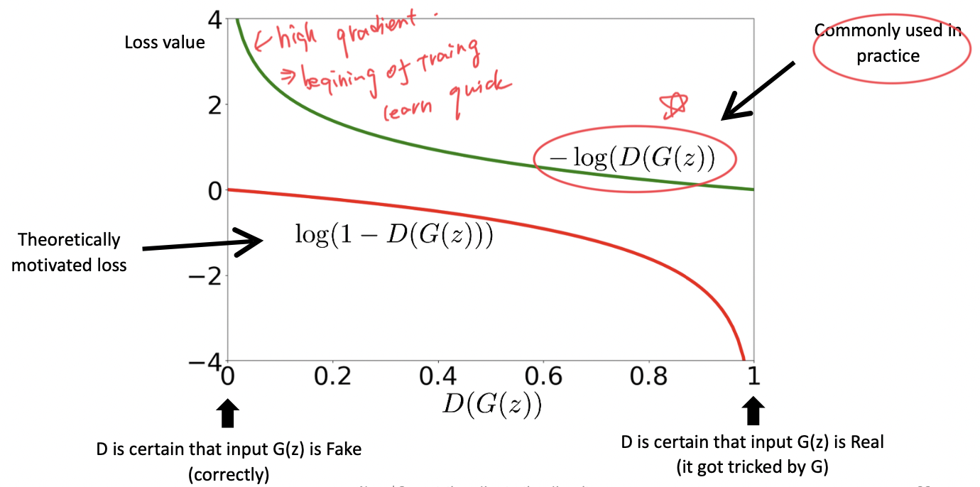
- We use different loss functions for the generator. Because with the original
logloss the network may stop learning from bad fake samples because it is sure they are bad (logloss is0which means no gradient). For good real samples we would get big gradients and we would try to improve network even more. But what we want is to learn from bad rather than good samples. We substitute:
\(\log(1-D_{\phi}(G_{\theta}(z)))\to -\log D_{\phi}(G_{\theta}(z))\)
GANs are really powerful for generating fake images and interpalation